What the FAQ

You have questions, too many of them. We have answers.

Why doesn't anything happen when I run show(...)?

Interpret’s visualizations are designed to work best in Jupyter notebook-like environments (like Jupyter notebook, VS Code, Colab, …). If you’re running show() from a command line script, you may not be able to render visualizations directly – check the printed console output for a link to open in a browser.

By default, interpret hosts visualizations on a local web server using Plotly Dash. In some restricted environments, where applications are not allowed to host a local web server, we embed visualizations directly into the notebook. If Interpret did not automatically detect and switch the rendering mode, you can manually embed visualizations in restricted environments with the following code:

from interpret.provider import InlineProvider
from interpret import set_visualize_provider

set_visualize_provider(InlineProvider())

The InlineProvider is compatible with a broader range of environments than the default rendering logic in Interpret. However, warning: you may experience slower performance when calling show(), and the full interpret dashboard is currently unsupported with InlineProvider.

How do I generate the full interpret dashboard instead of the small single-explanation dropdown?

Make sure you are passing in a list of explanations to show. Note that you can also pass in a single explanation wrapped in a list. Ex:

from interpret import show

show(ebm_local)   # Returns small dropdown
show([ ebm_local ]) # Produces interpret dashboard

How can I extract the underlying data used to visualize explanations?

Every explanation object in interpret supports a .data() method, which returns a JSON-compatible dictionary of the underlying data used to produce the visualizations. Most explanations contain many visualizations – for example, explain_local() calls will produce visualizations for each individual instance passed to the function. data takes in a single parameter which indexes the explanation object and returns the data used for that individual explanation (ex: explanation.data(0) returns the data used for the first visualization in the object). To return data used for all visualizations, use the -1 key (explanation.data(-1)).

How can I save an explanation graph to disk?

Every explanation graph is a Plotly object, and can be saved to disk using the camera icon in the UI:

or with the Plotly Static Image Export tools. You can access individual Plotly figures with:

ebm_explanation = ebm.explain_global()
plotly_fig = ebm_explanation.visualize(0)

For example, to save every graph in a global explanation to the “images” directory on disk:

ebm_global = ebm.explain_global()
for index, value in enumerate(ebm.feature_groups_):
    plotly_fig = ebm_global.visualize(index)
    plotly_fig.write_image(f"images/fig_{index}.png")

What does the 'density' at the bottom of each graph mean?

The density is a histogram describing the data distribution for that feature (estimated using any data passed into the explain_* methods). It is often useful to understand how much data is in each region of the feature space when visualizing an explanation – models can perform very differently with large and small samples.

Does interpret support explainability for image and text data?

Not yet, but keep an eye out for future releases!

How do I install just a single explainer without any other dependencies?

This is possible by installing directly from the interpret-core base package for advanced users. For example, if you want to install EBM without any other explainers, run the following codeblock below:

pip install interpret-core[required,ebm]

The various installation options provided by interpret-core are specified in the interpret-core setup.py file. The required tag is generally recommended for all installs.

Why aren't the feature names showing in graphs?

If you are passing a numpy array to an explainer, make sure that the feature_names property is set (either by passing at initialization, or manually setting before calling an explain function). This should work automatically when using pandas dataframes.

EBM

Should I be parameter tuning EBMs (and if so, what parameters should I tune)?

In general, the default parameters for EBMs should perform reasonably well on most problems. We recommend training a model with defaults and looking through the learned functions to catch abnormal behavior before parameter tuning – oftentimes, these graphs help indicate which parameters to tune. Here’s some general recommendations:

• To produce the best models, we generally recommend setting outer_bags and inner_bags to 25 or more each. This will significantly slow down the training time of the algorithm, and may be infeasible on larger datasets, but tends to produce smoother graphs with marginally higher accuracy.

• If you believe the models might be overfitting (ex: large difference between train and test error, or high degrees of instability in graphs), consider the following options:

  • Reduce max_bins for smaller datasets, to clump more data together.

  • Make the early stopping more aggressive by decreasing early_stopping_rounds and increasing early_stopping_tolerance.

• Conversely, for underfit models which appear too conservative, you can do the opposite of the previous suggestions – increase max_bins and make early stopping less aggressive. It might also be helpful to increase the total allowed max_rounds.

• If many of the included interaction terms are significant (e.g. learning large values or ranking highly on the overall importance list), there’s a chance the 10 interaction terms included by default is insufficient for your dataset. Consider increasing this number.

• For general tuning, we recommend sweeping max_bins with values between 32 and 1024, and max_leaves from 2 to 5. These improvements are normally marginal, but may help significantly on some datasets.

What does the error bar on an EBM graph mean, and how are they calculated?

The error bars are rough estimates of the uncertainty of the model in each region of the feature space. A large error bar means that the learned function may have changed substantially with minor changes to the training data, and indicates that the interpretation of the model in that region should be treated with more skepticisim.

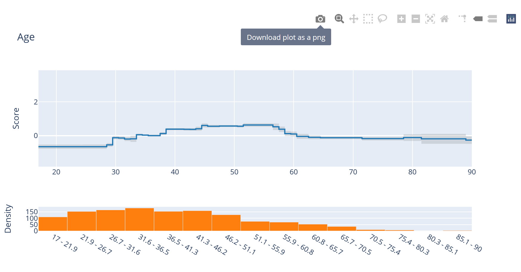
The size of the error bar is typically determined by two factors – the amount of training data in that region of the feature space, and the inherent uncertainty of the learned model. For example, consider this graph of the learned “Age” feature from the Adult income dataset:

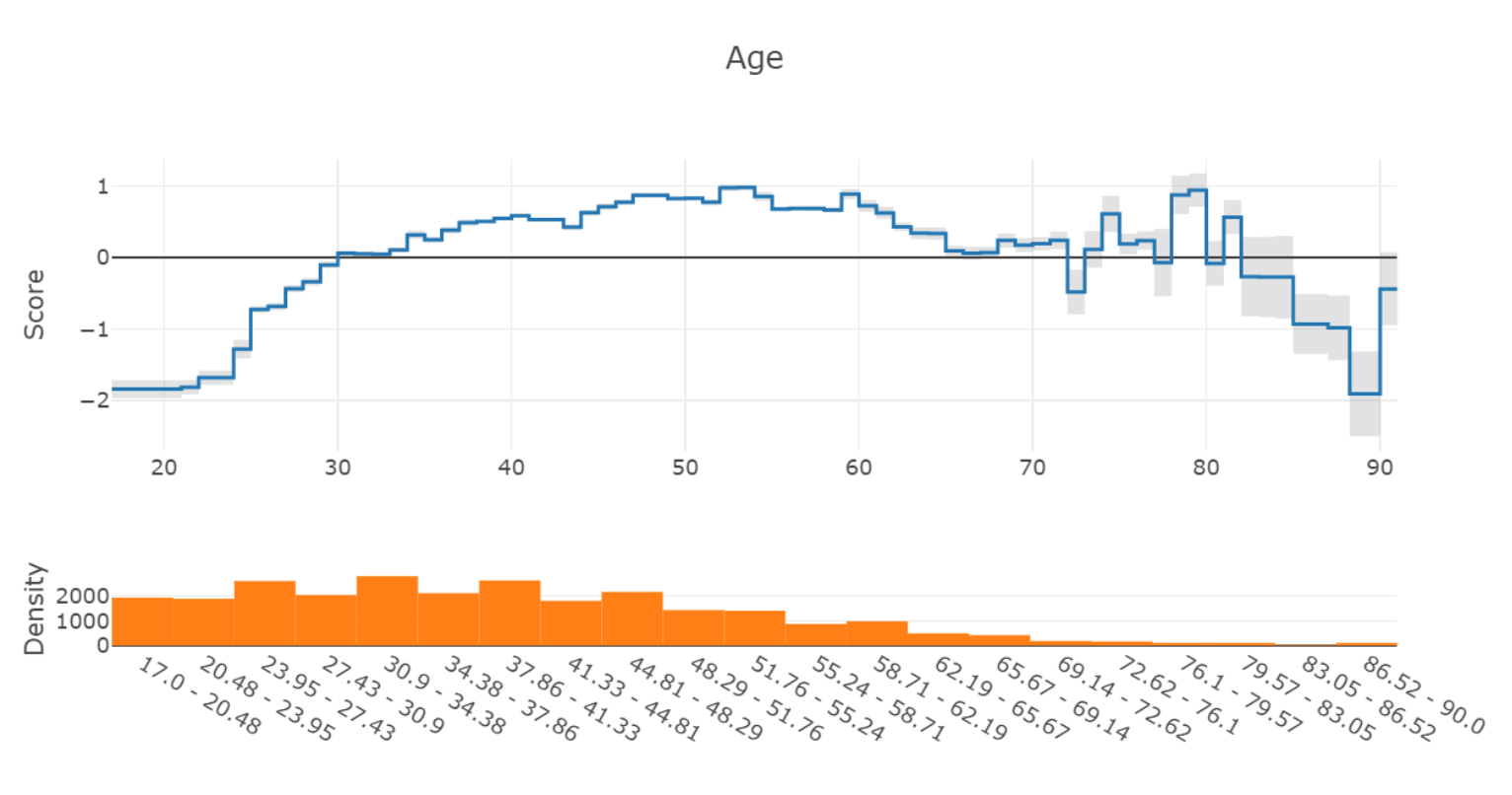
On the right side of the graph (Ages 70+), the model predictions become unstable, and the error bars become much larger to indicate this uncertainty. From the density graph at the bottom, we can see that this is likely due to the small number of samples in this area.

The error estimates are derived through bagging. By default, EBM trains 8 different mini-EBMs on random 85% subsamples of the training dataset. The number of mini-EBMs trained is controlled by the outer_bags parameter, and the proportion of data sampled is 1 - validation_size. The outputs of these models are averaged together to produce the final EBM, and the standard deviation of estimates for each region of the graph is published as the error bar. You can programmatically access the error bar sizes from the standard_deviations_ property on any EBM.

Do you have p-values for significance of EBM terms?

Not yet, though this is an area of active research. If you’re interested in discussing this or helping us figure it out, reach out!

What's the difference between EBMs in classification and regression?

The differences are largely analogous to the differences between linear regression and logistic regression. Like logistic regression, EBMs need to be adapted to the classification setting through the use of the logistic link function.

This link is used because probabilities are not additive – two features cannot each contribute +0.6 probability to a prediction, as the resulting final probability of 1.2 is undefined. The logistic link allows the models to train in the logit space – where the contribution of each feature can be additive – and convert back to a bounded probability at prediction time. Therefore, when interpreting the graphs of an ExplainableBoostingClassifier, it’s important to remember that the y-axis values are in logits. The interpretation of the shape is generally the same – positive values push the prediction towards a positive label for that class. However, because these graphs are in logarithm space, differences of +1 or +2 are quite significant.

In the regression setting, the interpretation is simpler: the y-axis values are directly in the units of the target. For example, if you are training on housing prices, the y-axis for each graph will represent exactly how many dollars that feature contributes to the final price of a model – no additional transformations needed!

How can I edit EBM models to remove unwanted learned effects?

The final EBM models are stored as numpy arrays in the terms_scores_ property. Indexing this array returns the function learned for a specific term in the EBM – for example, ebm.terms_scores_[0] will return the array for the first term. Editing this array directly will change all predictions made by the model for that corresponding region of the graph. A nicer API for this with more granular controls will be introduced shortly!

Can we enforce monotonicity for individual EBM terms?

We currently cannot do this through training, but it is possible to enforce monotonicity through postprocessing a graph. We generally recommend using isotonic regression on each graph output to force positive or negative monotonicity. Code examples coming soon!

How can we serialize EBMs and use them in production?

For full functionality, we recommend using pickle to serialize and deserialize EBM objects. Explanations can be serialized as JSON through the data method.

Thanks to Github user @MainRo, there is now an ebm2onnx package available which enables high speed inference on EBM objects through ONNX compatible runtimes. Check out the package here: SoftAtHome/ebm2onnx and install from PyPi via pip install ebm2onnx

Support

I need help, how do I get in touch?

For most questions we recommend raising a GitHub issue. Solving issues on GitHub means that other users like yourself can benefit from the same solutions. For anything else (or questions that need to be kept private), feel free to send us an email at interpret@microsoft.com .

I have a great idea, how can I contribute?

If you have code you’d like to commit, make sure you read the contributing guidelines, and send us a pull request.

If you’d like to request a new feature or discuss any ideas, just raise a GitHub issue.