Shapley Additive Explanations#
Link to API Reference: ShapKernel
See the backing repository for SHAP here.
Summary
SHAP is a framework that explains the output of any model using Shapley values, a game theoretic approach often used for optimal credit allocation. While this can be used on any blackbox models, SHAP can compute more efficiently on specific model classes (like tree ensembles). These optimizations become important at scale – calculating many SHAP values is feasible on optimized model classes, but can be comparatively slow in the model-agnostic setting. Due to their additive nature, individual (local) SHAP values can be aggregated and also used for global explanations. SHAP can be used as a foundation for deeper ML analysis such as model monitoring, fairness and cohort analysis.
How it Works
Christoph Molnar’s “Interpretable Machine Learning” e-book [1] has an excellent overview on SHAP that can be found here.
The conceiving paper “A Unified Approach to Interpreting Model Predictions” [2] can be found on arXiv here.
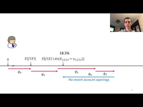
If you find video as a better medium for learning the algorithm, you can find a conceptual overview of the algorithm by the author Scott Lundberg below:

Code Example
The following code will train a blackbox pipeline for the breast cancer dataset. Aftewards it will interpret the pipeline and its decisions with SHAP. The visualizations provided will be for local explanations.
import numpy as np
from sklearn.datasets import load_breast_cancer
from sklearn.model_selection import train_test_split

from sklearn.ensemble import RandomForestClassifier
from sklearn.decomposition import PCA
from sklearn.pipeline import Pipeline

from interpret import show
from interpret.blackbox import ShapKernel

seed = 42
np.random.seed(seed)
X, y = load_breast_cancer(return_X_y=True, as_frame=True)
X_train, X_test, y_train, y_test = train_test_split(X, y, test_size=0.20, random_state=seed)

pca = PCA()
rf = RandomForestClassifier(random_state=seed)

blackbox_model = Pipeline([('pca', pca), ('rf', rf)])
blackbox_model.fit(X_train, y_train)

shap = ShapKernel(blackbox_model, X_train)
shap_local = shap.explain_local(X_test[:5], y_test[:5])

show(shap_local, 0)
Using 455 background data samples could cause slower run times. Consider using shap.sample(data, K) or shap.kmeans(data, K) to summarize the background as K samples.
Further Resources
Bibliography
[1] Christoph Molnar. Interpretable machine learning. Lulu. com, 2020.
[2] Scott Lundberg and Su-In Lee. A unified approach to interpreting model predictions. arXiv preprint arXiv:1705.07874, 2017.
